
Coaxial Cable Fields
Jan 07, 2013
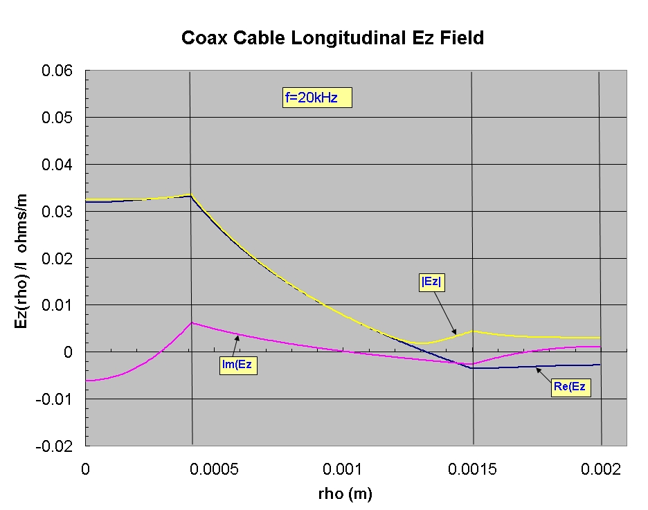
The graphs below show accurate calculations of the longitudinal (axial) electric field profiles Ez(ρ) for the circular symmetric principal TM propagation mode
in typical coaxial cable at frequencies of 1 MHz and 20 kHz.
The plots display the ratio of the complex Ez(ρ) field value divided by the total current I (integrated in the cross-section) at a fixed value of z. The current I in inner and outer conductors are, for any frequency,
almost exactly identical (but reversed in sign) assuming that the conductors are typical conductors with high conductivity and the dielectric is a typical dielectric with low shunt conductance.
Daywitt (1991) discusses the accuracy of this approximation.
The familiar lateral directed fields Hφ(ρ) and Eρ(ρ) are much simpler in form and in the dielectric between the conductors have an almost exact 1/ρ lateral dependence.
Plotting Ez(ρ)/I which is in units of Ω/m, is useful because the values of this quantity at Ri (the radius of the inner solid conductor) and at Ro (the inner radius of the
outer tubular conductor) are just the distributed internal impedances (or surface impedances) for each conductor.
The real and imaginary parts are simply the series resistances and (inductive) reactance of the corresponding conductors. When the external distributed
inductive reactance is added to these, the result is Z the total distributed series impedance which is the same quantity used in
the standard transmission like formalism (this is easy to show from Maxwell's equations as demonstrated, for example, by Schelkunoff 1934).
The longitudinal current density at any point in the conductors is just the conductor conductivity times the Ez field at that point. Note that since the
Ez field is complex, this means that there is a phase shift effect in the Ez field as a function of the radial distance ρ.
The plots show the real and imaginary parts and the magnitude of Ez(ρ). These plots represent the Ez component's field amplitude dependence on ρ for a wave
propagating in the + z direction.
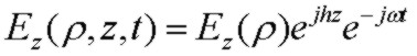
The complete field dependence for this component of the field, including the temporal and z (propagation direction) dependence is:

where α is the attenuation coefficient and β is the phase constant. These parameters and the fields are all determined by the conductor and
dielectric properties as well as the dimensions of the coaxial cable structure. Note that some authors (Stratton, Sommerfeld etc.) choose an alternate but equivalent sign convention
and definition of the axial "propagation constant" h as:

Exact Coaxial Cable Fields
The results shown above are based on the approach presented by Schelkunoff (1934) in which it is assumed that the total current in the outer conductor is identical (but opposite in direction)
to that carried by the inner conductor. Also, the results assume that the displacement current in the conductors is completely negligible compared to the conduction current. This allows
application of Ampere's law (neglecting the displacement current contribution) relating magnetic field at any radius to the interior current at that radius. This approach produces very accurate results for the field shapes, including skin depth effects in
both inner and outer conductors, and propagation constant (phase velocity and attenuation) for any realistic coaxial cable.
However, at low frequencies where the Ez field penetrates to the outer region of the outer conductor, there will be field penetration (leakage) OUTSIDE of the coaxial cable. The results shown
above for 20kHz demonstrate field leakage outside the coax, since the Ez field is continuous across the boundary, but the limitation in the formalism doesn't permit a proper prediction of the fields OUTSIDE the coaxial cable.
Daywitt (1991) provides an exact formalism, including displacement current, which however assumes an infinite outer conductor. Daywitt includes a thorough discussion demonstrating that
the various approximations involving neglecting displacement current are excellent.
The results of Schelkunoff include a finite outer conductor thickness, but don't allow for proper determination of fields outside the outer conductor. It is possible to extend the general formalism
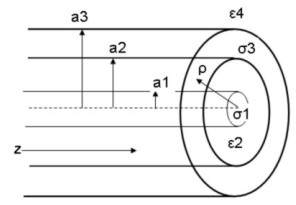
presented by Stratton (1941) to include a finite outer conductor thickness and an infinite final dielectric medium. The analysis then consists of matching tangential fields Ez and Hφ at
3 interfaces. As demonstrated by Stratton in a very general way, tangential field matching is exactly equivalent to matching radial impedances of the regions at the interfaces. Including
displacement current in all regions, this leads to a fairly complex transcendental equation with the roots being the axial propagation constants h. As usual there are an infinite number of
such roots for the circular symmetric case, and as usual the root with the smallest propagation constant closest to the bulk propagation constant of the interior dielectric is the low-loss TM principal mode.
It is not difficult to perform a computational mesh search for h. The results for a typical coax with typical low-loss external dielectric produce results which are almost identical to
those predicted by the simpler Schelkunoff analysis. The plots below show the axial field Ez(ρ) and azimuthal magnetic field Hφ(ρz) for the same cable analyzed above for f=20kHz and
with an external dielectric constant of 1 and negligible loss.
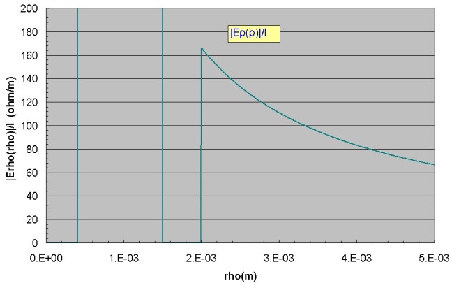
The substantial penetration of Ez beyond the outer region of the cable is evident with a slow drop off. Similarly, the radial component of electric field Eρ(ρ) which is much higher in value
will penetrate the outer dielectric. This field penetration at low frequencies will lead to coaxial cable crosstalk. Since
the field penetration is substantial, it is unlikely that the generator at one end of the coax will launch the principal mode exactly but the complex field at the generator, which will consist of a
superposition of many modes, including the nonpropagating evanescent modes, will quickly evolve (with propagation distance z) into the low-loss principal mode shown below:
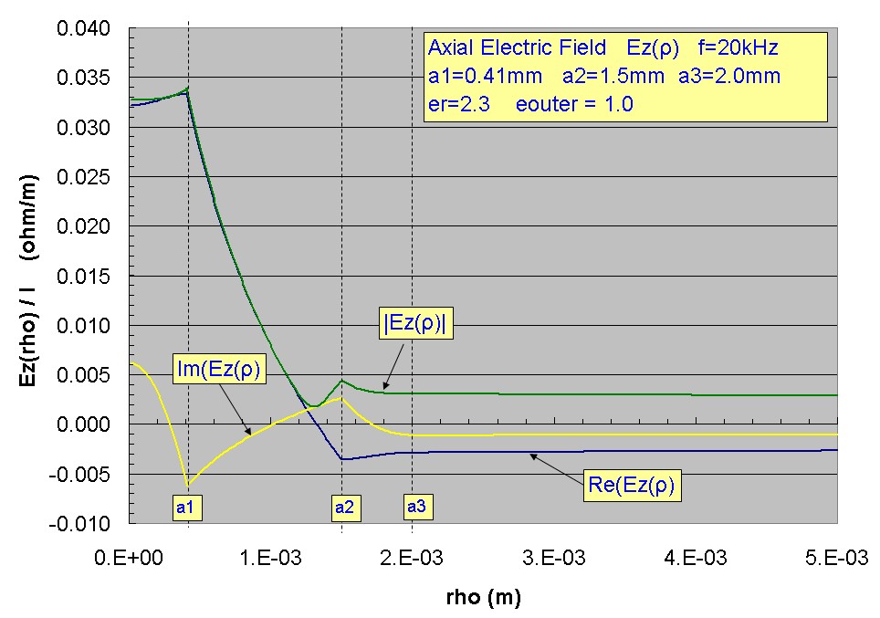
The fields within the outer conductor are almost identical to those calculated above using Schelkunoff's
approach. Note that the Im(Ez) is reversed in sign due to the sign convention (see above) used in Stratton's approach.
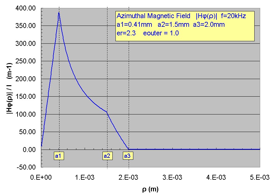
As expected the magnetic field H is almost exactly zero at the outer surface of the outer conductor, confirming that Ampere's law, not including the displacement current,
is almost exact and that the total current carried in outer and inner conductors is almost identical. There is however a weak magnetic field that extends outside the outer conductor,
and consequently the radial electric field extends outside.
The magnetic induction B (Tesla) is related to the magnetic field H (Ampere/m) by B = μoH where μ = 4πx10-7H/m.
Inside the conductors the electric field vector is almost perfectly axial (z direction) and in the dielectric regions, the electric field is almost perfectly radial (see Sommerfeld (1952) for an excellent
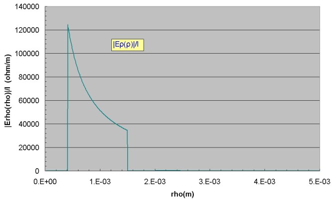
discussion of this). The component of radial electric field Eρ(ρ) is shown below with a magnified view showing the field penetration into the outer dielectric region. In the conductors
the radial electric field is extremely small (~ 1e-9 ohm/m for this example) compared to the axial electric field of ~ 1e-3 ohm/m in the outer conductor. Conversely, in
the dielectric regions, it is seen that the radial electric field is much greater than the axial electric field. The shape of Eρ(ρ) in each region is identical to that of Hφ(ρ).
However, there is a large discontinuity in Eρ(ρ), which is normal to each interface, at each conductor/dielectric interface. This means that a surface charge exists in the conductor at each interface with a surface charge density value given by δ = εEρ(ρ=ρi)
in Coulomb/m^2 where ε and Eρ are the dielectric constant and radial electric field in the dielectric next to the conductor. This surface charge layer (on both inner and outer conductors) is
propagated as a wave in the z direction exactly as the fields themselves:
Characteristic Impedance Zo, Distributed Series Impedance Z and Distributed Shunt Admittance Y
The transmission line parameters Zo, Z and Y can be accurately determined from the axial propagation constant h found above (using Stratton's sign convention and definition of h above) and radial electric field Eρ(ρ). The
definition of characteristic impedance Zo for the waveguide is:
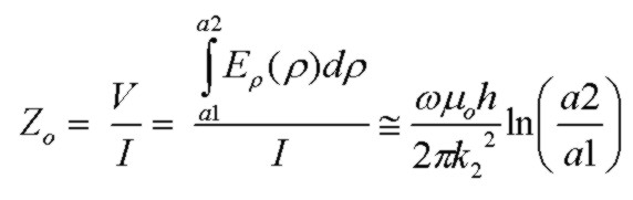
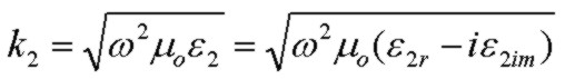
where k22 is the bulk propagation constant for medium 2 (the dielectric medium between conductors):
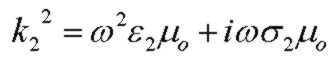
where ε2 and σ2 are the dielectric constant and conductivity (usually very small) in the dielectric medium between the conductors.
Zo will be complex since Eρ(ρ), h and k22 are all in general complex at any frequency.
Using the analytical expressions for Eρ(ρ) involving Bessel functions, it is easy to compute Zo exactly (given the numerical solution for the axial propagation constant h). However the approximate result
above for Zo is found to be very accurate for all cases of interest. Given Zo and h, the other transmission line parameters are easily calculated from:

where Z is the distributed series impedance (ohms/m) which consists of real and imaginary parts representing the line distributed series resistance and line distributed series inductive reactance.
Y is the distributed shunt admittance (mhos/m) consisting of real and imaginary parts representing the line shunt conductance G (mhos.m) (usually very small due to residual conductivity in dielectric medium 2)
and shunt distributed capacitance C (Farads/m) .
Full Frequency Range Formulae
The results above presented full accuracy computations for the propagation constant and fields of the principal TM mode for coaxial cable with a finite thickness outer conductor at any frequency. For extended
computational purposes, it is convenient to have an accurate closed form solution valid over all frequency. Daywitt (1991) provided a full-frequency range closed-form expression for the propagation constant,
for the case of infinite outer conductor thickness, originally published by Stratton (1941) and provided a comprehensive comparison with exact results demonstrating the high accuracy
of the approximate expression. A study of Schelkunoff's (1934) expressions, derived using a more intuitive approach using "surface impedances" concepts for coaxial cable
with a finite thickness outer conductor shows that the approximations involved (neglecting displacement current in the conductors etc.) are identical to those used in Daywitt's approximate expression.
Therefore a full frequency range expression WITH A FINITE THICKNESS OUTER CONDUCTOR with similar accuracy to that of Daywitt/Stratton's approximate expression can be obtained.
(Note: In the sections below h is the transverse propagation constant in the dielectric medium).
Using Schelkunoff's sign convention (identical to that of Daywitt) and for non-magnetic media:
the distributed line impedance Z (Ω/m), which includes all resistive and reactive components, is found to be:
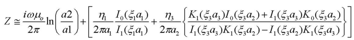
which for high frequency or very thick outer conductor a3>>a2 reduces to the case with infinite outer conductor thickness:
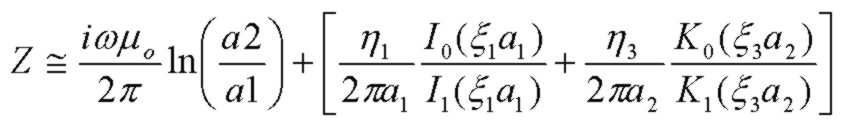
where the Bessel function parameters for I and K Bessel functions are:
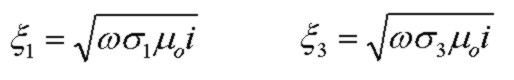
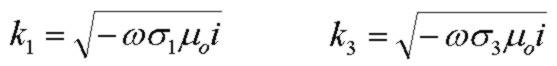
and the intrinsic impedances η of inner and outer conductors are :
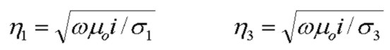
and the material propagation constants in the conductors (ignoring the negligible displacement currents) and inner dielectric (which may contain loss) are:
Note that the full-range expression for Z above does NOT include the material constants of the OUTER dielectric medium. This is due to the fundamental assumption that the conductivity of the outer conductor is
so high that displacement current can be neglected in the conductors which also means that the total current in the outer conductor is identical to very high precision to that of the inner conductor. This also
implies using Ampere's law (as demonstrated above) that the magnetic field H is very nearly zero at the outer surface of the outer conductor. Even though there is some field penetration outside the outer conductor particularly
at low frequency, the propagation characteristics of typical coax cable with a finite outer thickness conductor are completely controlled by the material constants of the inner and outer conductors and the inner dielectric between
the conductors. Of course, if the outer dielectric medium has very high loss and at lower frequency with field penetration beyond the outer conductor, this must eventually lead to an increase in the principal mode propagation loss.
In this case, the extra loss introduced by the outer infinite dielectric medium can be determined by solving for the exact propagation constant using the full transcendental root equation discussed above.
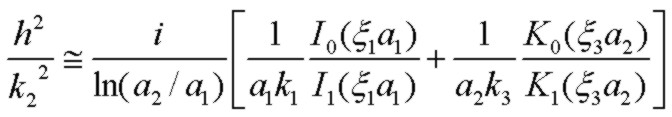
The full-frequency-range TRANSVERSE propagation constant h in the dielectric region between the conductors (identical to h in Daywitt's work of Jo(hρ) and λ2 in Stratton) for finite thickness
outer conductor is found to be:
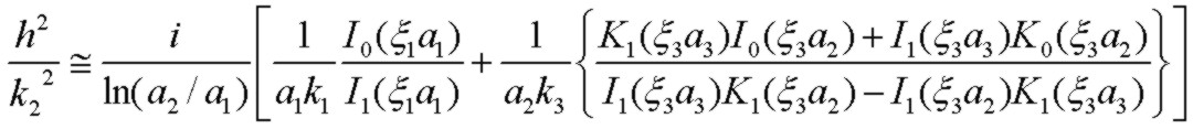
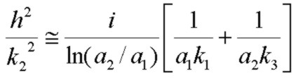
which for high frequency or very thick outer conductor reduces to the case with infinite outer conductor thickness:
This is equivalent to Daywitt's approximation (35).
Note that Schelkunoff uses modified Bessel functions I and K while Daywitt uses Bessel functions J and Y (or N) which are equivalent. At high frequency,
the microwave approximation is recovered with Io/I1 --> 1 and Ko/K1 --> 1 which yields the usual high-frequency result:
The axial progagation constant Γ is obtained from:
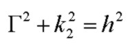
The real and imaginary parts of Γ are the attenuation coefficient α and phase constant β, and the phase velocity is vp:
The characteristic impedance Zo is obtained from:
where:
with the approximate value for Y being highly accurate for all cases of interest. As is usually the case, the dielectric loss is extremely low and G << i*ωC. Since C is to a very good approximation independent of frequency and
equal to the low frequency capacitance per length, it is possible to experimentally determine Zo accurately at any frequency from a measurement of the propagation constant Γ as demonstrated
by Marks and Williams (1991).
A comparison of results obtained by solving the exact transcendental equation for the propagation constant root and the full-range approximations above for Zo and h at sample
frequencies indicate that the approximation is valid to at least 1 part in 1E5 from DC to GHz. Schelkunoff provides various approximations for the Bessel function expressions above. However, there
are high-precision libraries of Bessel functions available for computation. Alternately, it is not difficult to create high-precision libraries of the necessary Bessel functions for arbitrary complex arguments.
Coaxial Line versus Single "Wire Wave" Line Principal TM Wave
The full frequency range approximate expressions above for the transverse propagation constant h2 in the dielectric between the inner and outer conductors
due to Daywitt/Stratton and the extended version provided above for the case of finite thickness outer conductor are extremely accurate for all realistic coaxial cable geometries
and for frequencies from DC to several GHz provided that the frequency-dependent dielectric constant is properly specified.
A basic assumption used in deriving these full-frequency range expressions is h*ρ<<1 in the dielectric medium between inner and outer conductor. This is an extremely
good approximation for all realistic coaxial geometries. Nevertheless, it is interesting to study the transition to the well known "wire-wave" line as the limiting case of a coaxial line with a2 --> ∞.
Inspection of the expression for h above indicates that as a2 --> ∞, h-->0 and thus Γ --> i*k2. If the dielectric medium with material constant k2 is lossless, this implies that the principal
mode in this limit would have zero loss (the real part of Γ) which is incorrect since the principal TM wave for the single-wire line has finite loss due to the wire losses. This incorrect limiting
behavior is due to the assumption h*ρ<<1. It is well known (e.g. Stratton (1941)) that the propagation constant for the principal TM wave of the single-wire line is given exactly by the
smallest root of the determinantal equation:
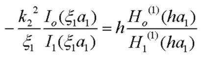
where all parameters are the same as in the previous section.
In solving for the propagation constant of the single-wire line, no assumptions need be made about the magnitude of h in the external dielectric medium. It is easy to solve for h
and Γ in this case using a rapidly-convergent iterative method described by Sommerfeld (1952).
The wire-wave determinantal equation above is derived as usual by field-matching of Ez and Hφ at the single interface at a1. It can also be derived
from the more complex transcendental equation for the coax line with the limiting simplifications associated with a2 --> ∞ but WITHOUT assuming h*ρ<<1.
Results comparing the axial propogation constant Γ and attenuation for a copper conductor line (σ=5.75e7 mhos/m) with lossless air dielectric at f=1MHz are:
Coaxial Line:   a1=1mm  a2=5mm  ε2=(1.0, 0)
Γ=(2.6310e-4 + j2.1217e-2) m-1       α=2.2853e-3 dB/m

WireWave Line:  a1=1mm  ε2=(1.0, 0)
Γ=(2.6922e-5 + j2.0983e-2) m-1       α=2.3384e-4 dB/m
where the loss for wirewave line is the minimum loss value at 1 MHz as the radius of the outer conductor of the coax guide tends to infinity.
Reference:
- The Electromagnetic Theory of Coaxial Transmission Lines, S. Schelkunoff, 1934, Bell System Technical Journal, p. 532
- Exact Principal Mode Field for a Lossy Coaxial Line, W. C. Daywitt, IEEE Trans. MTT, v39, #8, 1991 p. 1313
- Electromagnetic Theory, J. Stratton, 1941, McGraw Hill, pp. 551-554
- Electrodynamics, A. Sommerfeld, Lectures on Theoretical Physics, VIII Academic Press, 1952
- Fields and Waves in Communication Electronics, S. Ramo, J. Whinnery and T. Van Duzer, 2nd Edn. 1984, John Wiley & Sons, pp. 249-252
- Inductance Calculations, F. Grover, 1946, 1973, Dover, Instrument Society of America, p. 42, pp.262 - 282
- Waveguide Handbook, N. Marcuvitz, 1986, Peter Peregrinus Ltd. pp. 17-25, p. 72
- Characteristic Impedance Determination Using Propagation Constant Measurement, R. Marks and D. Williams, IEEE MGW Letts, v1, #6, 1991 p. 141