Characteristic Impedance Calculation For Typical RG58U Coaxial Cable
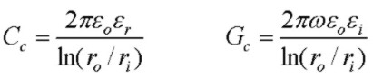
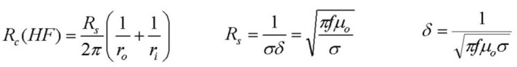
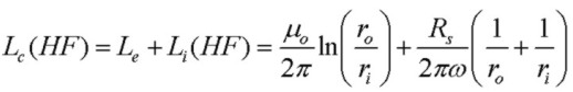
The plots below show the characteristic impedance Zo for a coaxial cable with typical RG58U characteristics (cables from different manufacturers differ somewhat in the exact physical dimensions,
dielectric constants etc..) using the high and low frequency approximations above for Rc and Lc. The magnitude and phase of Zo are shown.
The "nominal" high frequency value of characteristic impedance is Zo = Sqrt(Le/Cc) = 51.3 Ohm for the dimensions shown.
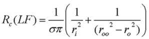
The parameters are shown in the inset of the graph along with the low frequency limits for Rc and Lc.
Two sets of curves are shown. The HF (blue) curves show the predictions based on the high-frequency expressions above which are therefore accurate only for f >~ 1MHz. The LF curves (yellow)
use expressions with the fixed limiting values of Rc and Lc and are therefore accurate for f < ~ 20 kHz.
The transition region between 20 kHz and 1 MHz will correspond to points intermediate between the two graphs. A comparison with exact data shows that for this example Zo follows the
LF approximate curve almost exactly up to ~ 100kHz and follows the HF approximate curve almost exactly for f > 100 kHz.
Accurate values require use of accurate Bessel function expressions (e.g. Schelkunoff, 1934).
Some values from the curves are: Zo (nominal) == Sqrt(Le/Cc) = 51.3 Ohm
Zo(100MHz) = 51.5 / -0.2 deg Ohm
Zo(1MHz) = 53.3 / - 2.1 deg Ohm
Zo(1kHz) = 240 / -43 deg
The second graph
shows the skin depth for copper as a function of frequency.


Special Cases:
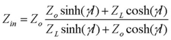
Given the characteristic impedance Zo at any frequency, the input impedance of any length of cable terminated with arbitrary complex impedance can be easily calculated
using the transmission-line transformation expression for Zin above. Two cases of interest are:
- short lengths of cable (l << wavelength) terminated with infinite load (open end cable)
- short lengths of cable (l << wavelength) terminated with a short circuit
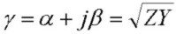
where wavelength = 2π/β and β is the phase constant.
Using the general expression above for Zin, these two cases have corresponding input impedances of:
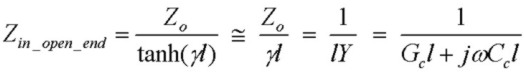

For the open-ended line, Gc is always << ωCc (since εi << εr for insulating dielectrics). Therefore the input impedance of a short length of cable is just the impedance of a capacitor of value Ccl.
This familiar result is therefore a very good approximation at ANY frequency.
For the shorted line, the situation at low frequency is different from high frequency. At high frequency, jωLcl becomes much greater than Rl and in this high-frequency limit, the input
impedance of the short shorted line is simply jωLcl, purely inductive with an inductance value of Lcl, another familiar result for high frequency.
However, at low frequency, the Rc and Lc both approach constant values (as discussed above), but the inductive reactance continues to drop at low frequency. Eventually Rc will exceed ωLc
and the input impedance of the shorted line will be resistive.
Using the same parameters as above for typical RG58U coaxial cable and a cable length of 3m (9' 10"), typical Zin values for these two cases are:
   Zin_open(1MHz) = 536.0 / -89.97 deg      ("capacitive")
   Zin_open(1kHz) = 537771.9  / -89.97 deg  ("capacitive")

   Zin_short(1MHz) =  5.31 / +85.8  deg      ("inductive")
   Zin_short(1kHz)    =  0.107 / +3.33 deg   ("resistive")
Physical Components of Z:
Schelkunoff (1934) provides an excellent and insightful discussion of the components (internal and external) of the distributed coaxial cable serial impedance Z. The internal components (or "surface impedances")
consist of resistive (real) and reactive (imaginary) parts arising from current flow and magnetic flux created inside the inner and outer conductors of the coaxial cable. The resistive parts contribute
to power absorption and attenuation with distance along the cable.
In addition the external component of impedance originating from the magnetic field between the inner and outer conductors, is purely inductive and is described by the high-frequency inductance.
It is interesting to display the real and imaginary parts of each of these components.
The total distributed series impedance Z is the sum of the real and imaginary parts from each contributor, in units of Ω/m. The plot below shows the results of an accurate
calculation using the complete Bessel function field solutions. The plots are therefore accurate over the complete frequency range shown.
The usual engineering transmission-line equations can be derived directly from the fundamental field equations.
The graphs below show that for f > 20kHz, the total series impedance Z becomes dominated by the reactive part Z_im due to the dominance of the external inductance Le.
For f < 20 kHz, Z becomes resistive and (for the dimensions of conductors shown) dominated by the DC resistance of the inner conductor. The change in shape between 50kHz - 500 kHz
is due to the skin-depth effect. At low frequencies, current is uniformly distributed in the cross sections of both conductors. At high frequencies, current is confined to a very thin surface layer in both
conductors. This causes both the resistive part Z_re, which detemines attenuation, and the reactive part Z_im to increase with frequency. However the reactive part strongly dominates for f > 1MHz.
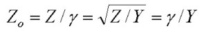
This leads to the characteristic impedance Zo = √(Z/Y) being almost resistive with a slight reactive component:

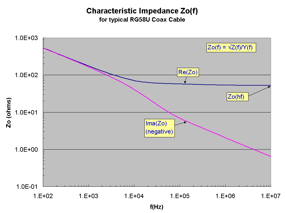
The plot below shows an exact calculation for the characteristic impedance Zo= √(Z/Y) using the same parameters as above. The real and imaginary parts of Zo are shown with the imaginary part being negative.
As expected, at high frequency, Zo becomes almost perfectly resistive with an asymptotic value Zo(hf) ~ √(Le/C) = 51.3 Ω. At low frequency, Zo becomes strongly complex
with equal resistive and reactive parts (phase angle -45 deg). The magnitude of Zo in this limit is √(Rdc/ωC), increasing with decreasing frequency. The transition region arising from
the skin-depth effect is evident between 10kHz and 100 kHz :
Reference:
- Fields and Waves in Communication Electronics, S. Ramo, J. Whinnery and T. Van Duzer, 2nd Edn. 1984, John Wiley & Sons, pp. 249-252
- Electromagnetic Theory, J. Stratton, 1941, McGraw Hill, pp. 551-554
- The Electromagnetic Theory of Coaxial Transmission Lines, S. Schelkunoff, 1934, Bell System Technical Journal, p. 532
- Inductance Calculations, F. Grover, 1946, 1973, Dover, Instrument Society of America, p. 42, pp.262 - 282.
- Waveguide Handbook, N. Marcuvitz, 1986, Peter Peregrinus Ltd. pp. 17-25, p. 72

 Coaxial cable is characterized by a "nominal" real characteristic impedance Zo such as 50 or 75 ohm. Zo generally is defined as the ratio of a sinusoidal AC voltage phasor
to the current phasor, which may be phase shifted, for a single outbound travelling wave (with no reflection from the cable end). The nominal Zo value refers to the high frequency RF value, appropriate to typical usage of this type of cable.
While this description is usually sufficient for frequencies above a few MHz, Zo is in general complex (reactive) and at lower frequency, the reactive nature of Zo becomes more apparent.
This is due to the frequency-dependent relative values of series resistance and inductance, combined with the skin-depth effect. Although complete solutions for Zo are available for any frequency
(e.g. Schelkunoff, 1934) , the general solutions involve complex Bessel functions which are difficult to analyze for frequency trends.
Instead, it is instructive to consider approximate solutions which are valid at either high or low frequency.
High frequency approximations are readily available (e.g. Ramo et. al. 1984). In addition, it is not difficult to calculate the frequency dependence of Zo at lower frequency, given the material properties and dimensions of the cable.
This note presents results of calculation for the Zo dependence on frequency of common RG58U "50 ohm" coaxial using high and low frequency approximate expressions.
Detailed field plots based on more comprehensive modelling for a typical coaxial cable quantify the field penetration outside of coax at low frequencies.
A 200 kHz reference example provides accurate reference data for all field components.
A script calculator accurately computes coaxial cable parameters discussed below and transmission line parameters for any frequency.
Coaxial cable is characterized by a "nominal" real characteristic impedance Zo such as 50 or 75 ohm. Zo generally is defined as the ratio of a sinusoidal AC voltage phasor
to the current phasor, which may be phase shifted, for a single outbound travelling wave (with no reflection from the cable end). The nominal Zo value refers to the high frequency RF value, appropriate to typical usage of this type of cable.
While this description is usually sufficient for frequencies above a few MHz, Zo is in general complex (reactive) and at lower frequency, the reactive nature of Zo becomes more apparent.
This is due to the frequency-dependent relative values of series resistance and inductance, combined with the skin-depth effect. Although complete solutions for Zo are available for any frequency
(e.g. Schelkunoff, 1934) , the general solutions involve complex Bessel functions which are difficult to analyze for frequency trends.
Instead, it is instructive to consider approximate solutions which are valid at either high or low frequency.
High frequency approximations are readily available (e.g. Ramo et. al. 1984). In addition, it is not difficult to calculate the frequency dependence of Zo at lower frequency, given the material properties and dimensions of the cable.
This note presents results of calculation for the Zo dependence on frequency of common RG58U "50 ohm" coaxial using high and low frequency approximate expressions.
Detailed field plots based on more comprehensive modelling for a typical coaxial cable quantify the field penetration outside of coax at low frequencies.
A 200 kHz reference example provides accurate reference data for all field components.
A script calculator accurately computes coaxial cable parameters discussed below and transmission line parameters for any frequency.